Free Debt Avalanche Payoff Planner Google Sheets Template

What is This Thing Anyway? (The "Big Picture")

Imagine you have a few different credit cards or loans (we'll call these your "debts"). Each one is like a little monster that keeps growing because of something called "interest." The Debt Avalanche method is a super-smart way to get rid of these monsters, starting with the one that's growing the fastest (the one with the highest interest rate).

This Google Sheet is your personal helper to:

1. See all your "debt monsters" in one place.

2. Figure out which monster to attack first (the one with the highest interest).

3. Show you exactly how much to pay on each monster every month.

4. Show you how quickly you can defeat all of them and how much money you'll save on interest by attacking the scariest ones first!

Why is the "Avalanche" Method Cool?

It's like rolling a snowball down a hill.

• You pay the minimum on most debts.

• You throw all your extra money at the debt with the highest interest rate.

• Once that debt is gone, you take ALL the money you were paying on it (its minimum + the extra) and add it to the payment for the next highest interest debt.

• Your payment for the new target debt becomes a BIGGER snowball (an avalanche!), and you knock out debts faster and faster, saving the most money on interest in the long run.

How This Sheet Works (The Magic Behind the Curtain)

This sheet has a few "pages" or "tabs" at the bottom:

1. Instructions & Setup (This Page!): You are here.

2. Debt Input: This is where YOU tell the sheet about your debts.

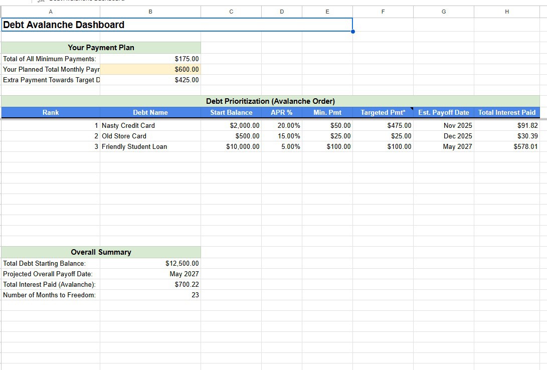
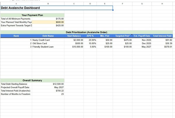
3. Avalanche Dashboard: This is your command center! It shows you the battle plan.

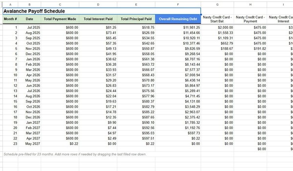
4. Avalanche Payoff Schedule: This shows you the fight, month by month, until all debts are gone.

Let's Get Started! (Your Action Steps)

Step 1: Tell the Sheet About Your Debts (Go to the "Debt Input" Tab)

• Click on the tab at the bottom called "Debt Input".

• You'll see columns like "Debt Name," "Current Balance ($)," etc.

• Only type in the light yellow boxes!

  • Debt Name: Give each debt a nickname (e.g., "Evil Visa Card," "Car Loan," "Student Loan #1").

  • Current Balance ($): How much you currently owe on that debt. Just type the number (e.g., 2000).

  • Annual Interest Rate (APR %): This is super important! Find this on your statement. If it's 20%, just type 20.

  • Minimum Monthly Payment ($): The smallest amount your lender says you have to pay each month. Type the number (e.g., 50).

• Do this for ALL your debts. The sheet has space for a few, and sample data is there to guide you. Just type over the samples with your real info.

Step 2: Decide Your Total War Chest (Go to the "Avalanche Dashboard" Tab)

• Click on the tab called "Avalanche Dashboard".

• Look for the section called "Your Payment Plan".

• Find the light yellow box next to "Your Planned Total Monthly Payment:".

• This is key: How much money can you afford to throw at ALL your debts combined each month?

  • For example, if you have $600 total to use for debt payments, type 600 here.

  • Important: This number must be at least as much as the "Total of All Minimum Payments" (which the sheet calculates for you just above it). The more you can pay, the faster you'll be debt-free!

Step 3: See Your Battle Plan! (Still on "Avalanche Dashboard")

Once you've done Step 1 and Step 2, the magic happens!

• Debt Prioritization (Avalanche Order):

  • The sheet automatically lists your debts here, but now they're sorted! The one with the highest APR % (scariest monster) is at the top (Rank 1). This is your first target!

  • Rank: Shows the attack order.

  • Debt Name, Start Balance, APR %, Min. Pmt: This is the info you entered, just sorted.

  • Targeted Pmt*:

    • For your Rank 1 debt, this shows its minimum payment PLUS all the "Extra Payment Towards Target Debt" (calculated in the "Your Payment Plan" section). This is the big punch you're throwing at the scariest monster!

    • For other debts, it will show just their minimum payment (for now).

  • Est. Payoff Date: This will fill in later! It will tell you when each debt is expected to be completely gone, based on the plan.

  • Total Interest Paid: This will also fill in later! It will show how much interest you'll end up paying for each specific debt under this plan.

• Overall Summary:

  • Total Debt Starting Balance: The grand total you owe right now.

  • Projected Overall Payoff Date: This will fill in later! It tells you the glorious day when ALL your debts will be gone!

  • Total Interest Paid (Avalanche): This will fill in later! Shows the grand total of all interest you'll pay across all debts using this awesome plan.

  • Number of Months to Freedom: This will fill in later! How many months until you're debt-free.

Step 4: Watch the Month-by-Month Fight! (Go to "Avalanche Payoff Schedule" Tab)

This tab is where the sheet does all the hard math, month by month. You don't usually need to change anything here, just watch the plan unfold!

• Each row is a month.

• Month # and Date: Tracks the timeline.

• Total Payment Made: This should match your "Planned Total Monthly Payment" from the Dashboard (unless you're on the very last payment).

• Total Interest Paid / Total Principal Paid (This Month): Shows how much of your total payment went to interest vs. actually reducing your debt.

• Overall Remaining Debt: The grand total you still owe after that month's payments. This number goes down each month – yay!

• Then, for EACH of your debts (e.g., "Nasty Credit Card - ...", "Old Store Card - ..."):

  • Start Bal.: What you owed on that specific debt at the beginning of the month.

  • Payment: How much of your total monthly payment went to this specific debt.

    • You'll see the Rank 1 debt gets its minimum + all the extra money.

    • Other active debts just get their minimums.

    • Once a debt is paid off (its "End Bal." becomes $0), the money that was going to it "avalanches" over to the next debt in line, making its payment bigger!

  • Interest: How much interest was charged on this debt for the month.

  • Principal: How much of the payment for this debt actually reduced its balance.

  • End Bal.: What you owe on this debt at the end of the month. Watch these go to $0.00!

The sheet is pre-filled for many months. You'll see the balances go down until "Overall Remaining Debt" hits $0.00. The rows after that will look empty or show "Jan 1900" – that just means the fight is over for those months!

How Some "Magic" Formulas Work (Simple Explanation):

You don't need to know this, but if you're curious:

• Sorting on the Dashboard (QUERY):

  • =IFERROR(QUERY('Debt Input'!A2:D, "SELECT A, B, C, D WHERE A IS NOT NULL AND B > 0 ORDER BY C DESC, B DESC", 0), "")

  • What it does: It's like telling the sheet, "Go to the 'Debt Input' tab. Grab all the rows where I entered a debt name and the balance is more than zero. Show me the Debt Name, Balance, APR, and Min Payment. But, sort them so the one with the biggest APR (column C) is on top! If two debts have the same APR, put the one with the bigger balance (column B) first."

• Calculating "Extra Payment" on Dashboard (B6):

  • =MAX(0,IFERROR(B5-B4,0))

  • What it does: "Take 'Your Planned Total Monthly Payment' (B5) and subtract the 'Total of All Minimum Payments' (B4). If the result is less than zero for some reason, just show 0." This is your extra firepower.

• Calculating "Targeted Pmt*" for Rank 1 Debt on Dashboard (F10):

  • =IF(B10<>"", E10 + IF(A10=1, $B$6, 0) ,"")

  • What it does: "If there's a debt name in B10: Take its minimum payment (E10). Then, IF its Rank (A10) is 1, ADD the 'Extra Payment' (from cell 

    BB

    6). Otherwise, add 0."

• Monthly Payment for Rank 1 Debt on Schedule (e.g., H3):

  • =IF($G3<=0, 0, MIN($G3+$I3, MAX(MinPmtD1Formula, TotalPlannedPmt - IF($L3>0,MinPmtD2Formula,0) - IF($Q3>0,MinPmtD3Formula,0) )))

  • What it does (Simplified): "If this debt (Debt 1) still has a balance (G3 > 0):

    1. Figure out how much money is available for this debt: Take the TotalPlannedMonthlyPmt, then subtract the minimums needed for Debt 2 (if it's active, L3>0) and Debt 3 (if it's active, Q3>0).

    2. The payment to Debt 1 will be the larger of its own minimum payment OR the amount calculated in step 1.

    3. BUT, don't pay more than what's actually needed to pay it off this month (Start Balance + Interest)."

  • This is the core of the avalanche – it makes sure the top debt gets all available extra cash.

• Subsequent Row Start Balance on Schedule (e.g., G4):

  • =IF($A4<>"",K3,"")

  • What it does: "If there's a month number in A4: The starting balance for Debt 1 this month (G4) is whatever its ending balance was last month (K3)." This carries the balance forward.

• Stopping the Schedule (e.g., A4 on Schedule):

  • =IF(F3<=0,"",A3+1)

  • What it does: "Look at the 'Overall Remaining Debt' from last month (F3). If it's zero or less, show nothing. Otherwise, show the next month number (A3+1)."

Linking the Schedule Back to the Dashboard (The "Pending" Stuff):

Once the Avalanche Payoff Schedule is fully calculated (all debts paid down to $0.00):

• Est. Payoff Date (Dashboard G10):

  • A complex formula like =IFERROR(INDEX('Avalanche Payoff Schedule'!$B$3:$B, MATCH(TRUE, ARRAYFORMULA(INDIRECT("'Avalanche Payoff Schedule'!" & CHOOSE(A10, "K", "P", "U") & "3:" & CHOOSE(A10, "K", "P", "U"))<=0.001), 0)), "")

  • What it does (Simplified): "Look at the Rank in A10. Based on that rank, find the correct 'End Bal.' column for that debt on the 'Avalanche Payoff Schedule' (K for rank 1, P for rank 2, etc.). Find the first row in that column where the balance is $0.001 or less. Then, go to column B (Date) of the schedule for that same row and show me that date."

• Total Interest Paid (Dashboard H10):

  • Another complex formula.

  • What it does (Simplified): "Similar to above, find the correct 'Interest' column for this debt on the schedule. Add up all the interest amounts in that column only for the months until this debt was paid off."

• Overall Summary Projected Payoff Date (Dashboard):

  • =IFERROR(INDEX('Avalanche Payoff Schedule'!$B$3:$B, MATCH(TRUE, ARRAYFORMULA('Avalanche Payoff Schedule'!$F$3:$F<=0.001), 0)), "Calculating...")

  • What it does: "On the 'Avalanche Payoff Schedule', look at the 'Overall Remaining Debt' column (F). Find the first row where this total debt is $0.001 or less. Show me the date from column B for that row."

• Overall Summary Number of Months (Dashboard):

  • =IFERROR(MATCH(TRUE, ARRAYFORMULA('Avalanche Payoff Schedule'!$F$3:$F<=0.001), 0), "Calculating...")

  • What it does: "On the schedule, find the row number where 'Overall Remaining Debt' (column F) first hits $0.001 or less. That row number tells us how many months it took (since data starts on row 3, this is roughly the number of months)."

That's It!

You just need to do Step 1 and Step 2. The sheet does the rest of the heavy lifting.
Watch the Avalanche Dashboard and Avalanche Payoff Schedule to see your debt-destruction plan in action! The "Pending" fields on the Dashboard will fill up as the schedule calculates your path to being debt-free!

Good luck on your debt-free journey! You've got this!